Simulare Monte Carlo

A Monte Carlo method is a technique that involves using random numbers and probability to solve problems. The term Monte Carlo Method was coined by S. Ulam and Nicholas Metropolis in reference to games of chance, a popular attraction in Monte Carlo, Monaco (Hoffman, 1998; Metropolis and Ulam, 1949).

Computer simulation has to do with using computer models to imitate real life or make predictions. When you create a model with a spreadsheet like Excel, you have a certain number of input parameters and a few equations that use those inputs to give you a set of outputs (or response variables). This type of model is usually deterministic, meaning that you get the same results no matter how many times you re-calculate. [ Example 1: A Deterministic Model for Compound Interest ]

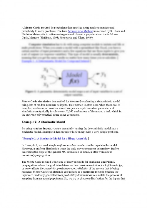
Figure 1: A parametric deterministic model maps a set of input variables to a set of output variables.

Monte Carlo simulation is a method for iteratively evaluating a deterministic model using sets of random numbers as inputs. This method is often used when the model is complex, nonlinear, or involves more than just a couple uncertain parameters. A simulation can typically involve over 10,000 evaluations of the model, a task which in the past was only practical using super computers.

Example 2: A Stochastic Model

By using random inputs, you are essentially turning the deterministic model into a stochastic model. Example 2 demonstrates this concept with a very simple problem.

[ Example 2: A Stochastic Model for a Hinge Assembly ]

In Example 2, we used simple uniform random numbers as the inputs to the model. However, a uniform distribution is not the only way to represent uncertainty. Before describing the steps of the general MC simulation in detail, a little word about uncertainty propagation:

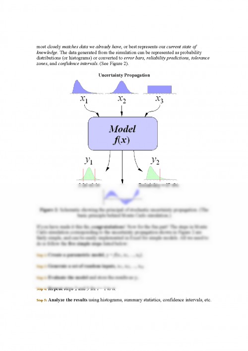
The Monte Carlo method is just one of many methods for analyzing uncertainty propagation, where the goal is to determine how random variation, lack of knowledge, or error affects the sensitivity, performance, or reliability of the system that is being modeled. Monte Carlo simulation is categorized as a sampling method because the inputs are randomly generated from probability distributions to simulate the process of sampling from an actual population. So, we try to choose a distribution for the inputs that most closely matches data we already have, or best represents our current state of knowledge. The data generated from the simulation can be represented as probability distributions (or histograms) or converted to error bars, reliability predictions, tolerance zones, and confidence intervals. (See Figure 2).

Uncertainty Propagation

Figure 2: Schematic showing the principal of stochastic uncertainty propagation. (The basic principle behind Monte Carlo simulation.)

If you have made it this far, congratulations! Now for the fun part! The steps in Monte Carlo simulation corresponding to the uncertainty propagation shown in Figure 2 are fairly simple, and can be easily implemented in Excel for simple models. All we need to do is follow the five simple steps listed below:

Step 1: Create a parametric model, y = f(x1, x2, , xq).

Step 2: Generate a set of random inputs, xi1, xi2, , xiq.

Step 3: Evaluate the model and store the results as yi.

Step 4: Repeat steps 2 and 3 for i = 1 to n.

Step 5: Analyze the results using histograms, summary statistics, confidence intervals, etc.

On to an example problem

Step 1: Creating the Model

We are going to use a top-down approach to create the sales forecast model, starting with:

Profit = Income - Expenses

Both income and expenses are uncertain parameters, but we aren't going to stop here, because one of the purposes of developing a model is to try to break the problem down into more fundamental quantities. Ideally, we want all the inputs to be independent. Does income depend on expenses? If so, our model needs to take this into account somehow.

We'll say that Income comes solely from the number of sales (S) multiplied by the profit per sale (P) resulting from an individual purchase of a gadget, so Income = S*P. The profit per sale takes into account the sale price, the initial cost to manufacturer or purchase the product wholesale, and other transaction fees (credit cards, shipping, etc.). For our purposes, we'll say the P may fluctuate between $47 and $53.

We could just leave the number of sales as one of the primary variables, but for this example, Company XYZ generates sales through purchasing leads. The number of sales per month is the number of leads per month (L) multiplied by the conversion rate (R) (the percentage of leads that result in sales). So our final equation for Income is:

Income = L*R*P

We'll consider the Expenses to be a combination of fixed overhead (H) plus the total cost of the leads. For this model, the cost of a single lead (C) varies between $0.20 and $0.80. Based upon some market research, Company XYZ expects the number of leads per month (L) to vary between 1200 and 1800. Our final model for Company XYZ's sales forecast is:

Profit = L*R*P - (H + L*C)

Y = Profits

X1 = L

X2 = C

X3 = R

X4 = P

Notice that H is also part of the equation, but we are going to treat it as a constant in this example. The inputs to the Monte Carlo simulation are just the uncertain parameters (Xi).

This is not a comprehensive treatment of modeling methods, but I used this example to demonstrate an important concept in uncertainty propagation, namely correlation. After breaking Income and Expenses down into more fundamental and measurable quantities, we found that the number of leads (L) affected both income and expenses. Therefore, income and expenses are not independent. We could probably break the problem down even further, but we won't in this example. We'll assume that L, R, P, H, and C are all independent.