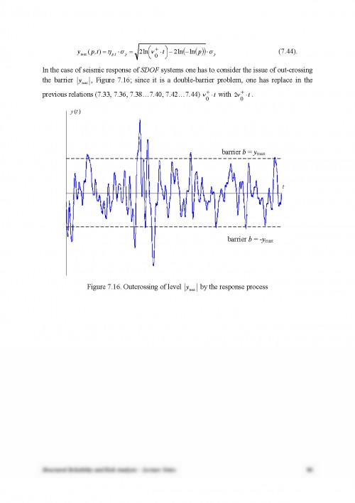
1.1. Data samples
If one performs a statistical experiment one usually obtains a sequence of observations. A typical example is shown in Table 1.1. These data were obtained by making standard tests for concrete compressive strength. We thus have a sample consisting of 30 sample values, so that the size of the sample is n=30.
Table 1.1. Sample of 30 values of the compressive strength of concrete, daN/cm2
320
380
340
350
340
350
370
390
370
320
350
360
380
360
350
420
400
350
360
330
360
360
370
350
370
400
360
340
360
390
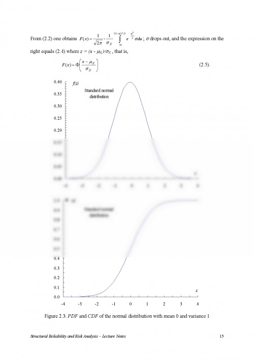
The statistical relevance of the information contained in Table 1.1 can be revealed if one shall order the data in ascending order in Table 1.2 (320, 330 and so on). The number of occurring figures from Table 1.1 is listed in the second column of Table 1.2. It indicates how often the corresponding value x occurs in the sample and is called absolute frequency of that value x in the sample. Dividing it by the size n of the sample one obtains the relative frequency listed in the third column of Table 1.2.
If for a certain value x one sums all the absolute frequencies corresponding to the sample values which are smaller than or equal to that x, one obtains the cumulative frequency corresponding to that x. This yields the values listed in column 4 of Table 1.2. Division by the size n of the sample yields the cumulative relative frequency in column 5 of Table 1.2.
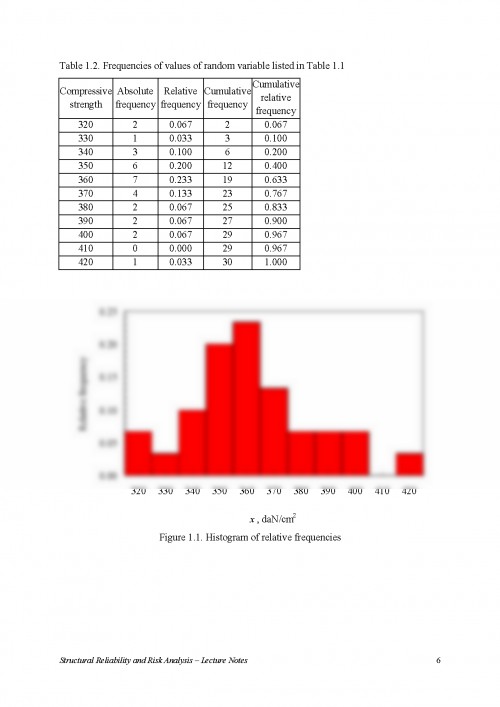
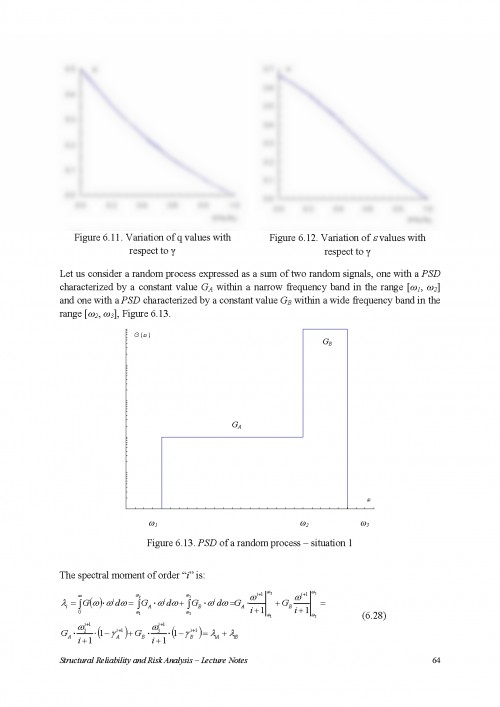
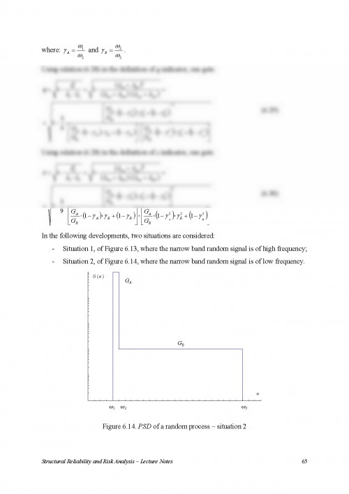
The graphical representation of the sample values is given by histograms of relative frequencies and/or of cumulative relative frequencies (Figure 1.1 and Figure 1.2).
If a certain numerical value does not occur in the sample, its frequency is 0. If all the n values of the sample are numerically equal, then this number has the frequency n and the relative frequency is 1. Since these are the two extreme possible cases, one has:
- the relative frequency is at least equal to 0 and at most equal to 1;
- the sum of all relative frequencies in a sample equals 1.
Structural Reliability and Risk Analysis - Lecture Notes 6
Table 1.2. Frequencies of values of random variable listed in Table 1.1
Compressive strength
Absolute frequency
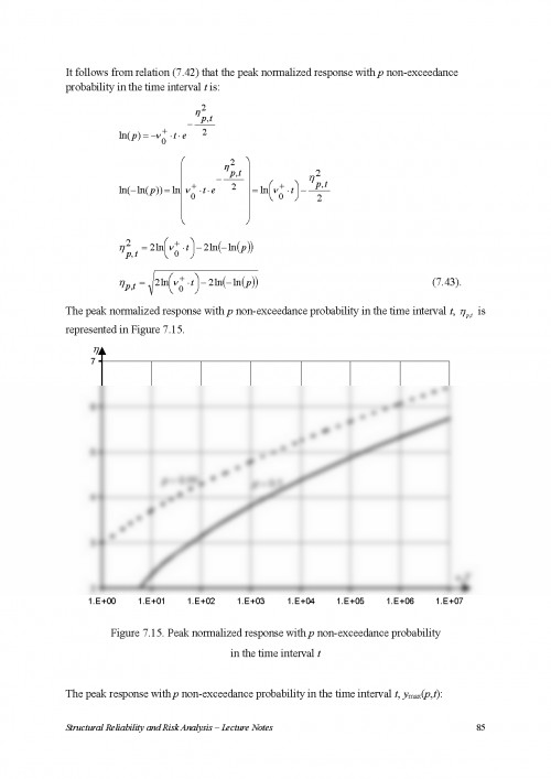
Relative frequency
Cumulative frequency
Cumulative relative frequency
320
2
0.067
2
0.067
330
1
0.033
3
0.100
340
3
0.100
6
0.200
350
6
0.200
12
0.400
360
7
0.233
19
0.633
370
4
0.133
23
0.767
380
2
0.067
25
0.833
390
2
0.067
27
0.900
400
2
0.067
29
0.967
410
0
0.000
29
0.967
420
1
0.033
30
1.000
0.000.050.100.150.200.25320330340350360370380390400410420x, daN/cm2Relative frequency
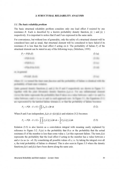
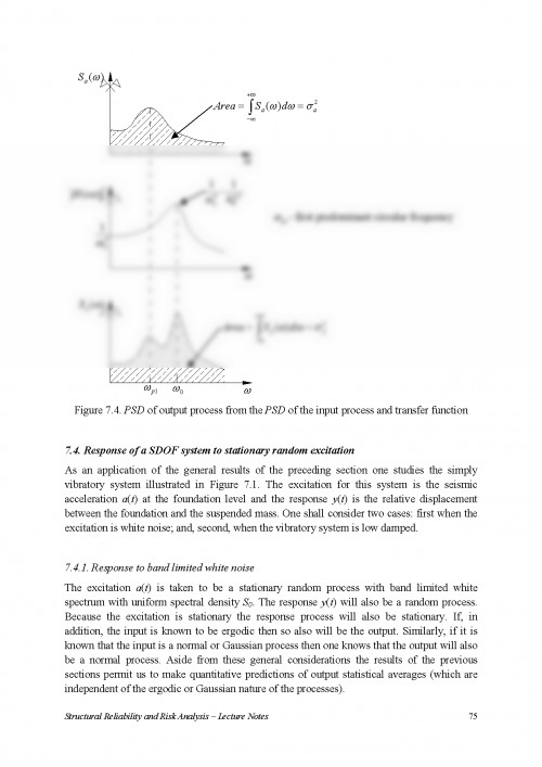
Figure 1.1. Histogram of relative frequencies
Structural Reliability and Risk Analysis - Lecture Notes 7
0.00.10.20.30.40.50.60.70.80.91.0320330340350360370380390400410420x, daN/cm2Cumulative relative frequency
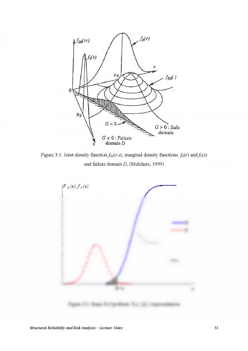
Figure 1.2. Histogram of cumulative relative frequencies
If a sample consists of too many numerically different sample values, the process of grouping may simplify the tabular and graphical representations, as follows (Kreyszig, 1979).
A sample being given, one chooses an interval I that contains all the sample values. One subdivides I into subintervals, which are called class intervals. The midpoints of these subintervals are called class midpoints. The sample values in each such subinterval are said to form a class. The number of sample values in each such subinterval is called the corresponding class frequency. Division by the sample size n gives the relative class frequency. This frequency is called the frequency function of the grouped sample, and the corresponding cumulative relative class frequency is called the distribution function of the grouped sample.
If one chooses few classes, the distribution of the grouped sample values becomes simpler but a lot of information is lost, because the original sample values no longer appear explicitly. When grouping the sample values the following rules should be obeyed (Kreyszig, 1979):
o all the class intervals should have the same length;
Aldea, A., Arion, C., Ciutina, A., Cornea, T., Dinu, F., Fulop, L., Grecea, D., Stratan, A., Vacareanu, R., 2004. Constructii amplasate in zone cu miscari seismice puternice, coordonatori Dubina, D., Lungu, D., Ed. Orizonturi Universitare, Timisoara 2003, , ISBN 973-8391-90-3, 479 p.
- Benjamin, J R, & Cornell, C A, Probability, statistics and decisions for civil engineers, John Wiley, New York, 1970
- Cornell, C.A., A Probability-Based Structural Code, ACI-Journal, Vol. 66, pp. 974-985, 1969
- Ditlevsen, O. & Madsen, H.O., Structural Reliability Methods. Monograph, (First edition published by John Wiley & Sons Ltd, Chichester, 1996, ISBN 0 471 96086 1), Internet edition 2.2.5 http://www.mek.dtu.dk/staff/od/books.htm, 2005
- EN 1991-1-4, Eurocode 1: Actions on Structures - Part 1-4 : General Actions - Wind Actions, CEN, 2005
- FEMA 356, Prestandard and Commentary for the Seismic Rehabilitation of Buildings, FEMA & ASCE, 2000
- Ferry Borges, J.& Castanheta, M., Siguranta structurilor - traducere din limba engleza, Editura Tehnica, 1974
- FEMA, HAZUS - Technical Manual 1999. Earthquake Loss Estimation Methodology, 3 Vol.
- Hahn, G. J. & Shapiro, S. S., Statistical Models in Engineering - John Wiley & Sons, 1967
- Kreyszig, E., Advanced Engineering Mathematics - fourth edition, John Wiley & Sons, 1979
- Kramer, L. S., Geotechnical Earthquake Engineering, Prentice Hall, 1996
- Lungu, D. & Ghiocel, D., Metode probabilistice in calculul constructiilor, Editura Tehnica, 1982
- Lungu, D., Vacareanu, R., Aldea, A., Arion, C., Advanced Structural Analysis, Conspress, 2000
- Madsen, H. O., Krenk, S., Lind, N. C., Methods of Structural Safety, Prentice-Hall, 1986
- Melchers, R. E., Structural Reliability Analysis and Prediction, John Wiley & Sons, 2nd Edition, 1999
- MTCT, CR0-2005 Cod de proiectare. Bazele proiectarii structurilor in constructii, 2005
Documentul este oferit gratuit,
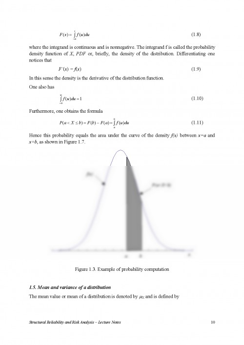
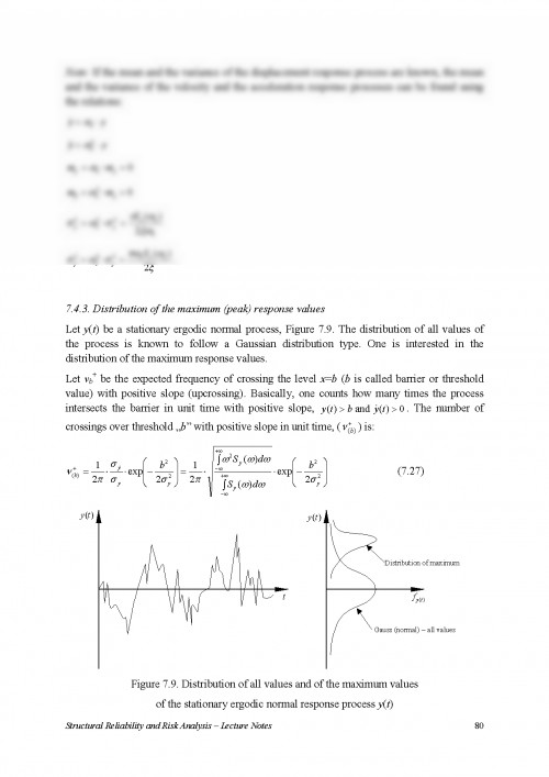
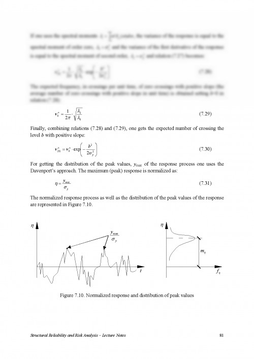
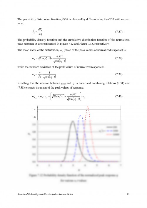
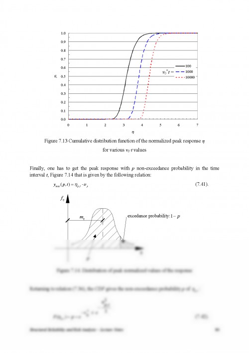
trebuie doar să te autentifici in contul tău.